Stationary Time Series for Pairs Trading Systems
A series of articles on using cointegration in a pairs trading system - Part 3 of 3
- Martyn Tinsley
- /
-
Abstract:
- Part 3 of our plain English guide to using cointegration within a pairs trading strategy. We explain the mathematics behind stationary time series.
This is Part 3 of ‘Cointegration for Pairs Trading’. I recommend you read Part 1 and Part 2 before continuing, so that the conetxt of this part is understood.
The mathematics behind stationarity for trading of cointegrated pairs
In order to study stationarity between two trading pairs, we will use what’s called an ‘autoregressive model of order one’ or AR(1) for short. “What?” I hear you say. An autoregressive model is simply one that requires a value in a time series to be related to a past value of itself in addition to some random error term. The fact that we will look at an AR model of order one, simply means that we only consider a lag of 1 value. So y at time t is related to y at time t-1. This can be written as:
yt = ρyt-1 + ε
where ρ represents a proportion of the previous value for y, and ε is an independent error term with zero mean. The important point is that if the absolute value of ρ is less than 1 then the series is said to be stationary (and will therefore return to the mean). The lower the value of ρ, the quicker and more efficiently it will return to the mean. If the absolute value of ρ equals 1 then the series is non-stationary. In this case we are left with a random walk where the price might return to its mean, but there is no guarantee it will do so.
|ρ| < 1 - Stationary
|ρ| = 1 - Non-Stationary
You can very easily test this in a spreadsheet yourself if you wish. This is a useful exercise to do because seeing is believing. However, if you are willing to trust me, this is what the time series look like for different values of ρ:
Three Examples for ρ=1 (non-stationary)
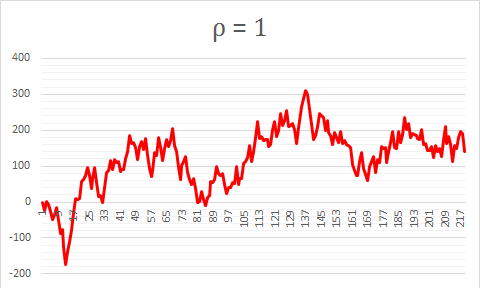
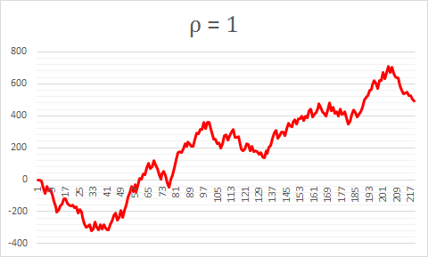
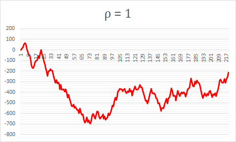
The reason each random walk is different is because of the randomness of the error term ε
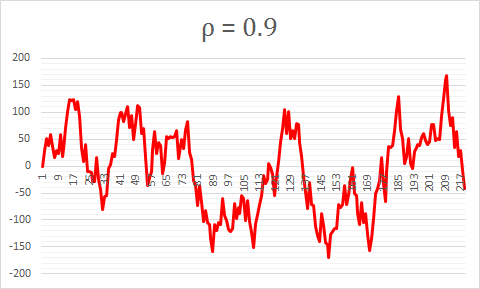
Example for ρ=0.9
Note how although this exhibits some characteristics of a random walk, it does eventually return to the mean. This propensity to revert to the mean will always be the case eventually, since |ρ| < 1
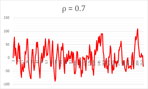
Example for ρ=0.7
Although the random walk characteristics still persist to a small extent, the propensity to revert to the mean is now much stronger
Example for ρ=0.4
Here, almost as soon as the series diverges from the mean, it reverts back.
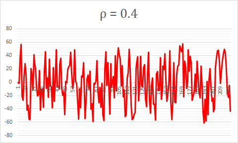
There will always be a propensity to revert to the mean when |ρ| < 1
Spurious Regressions
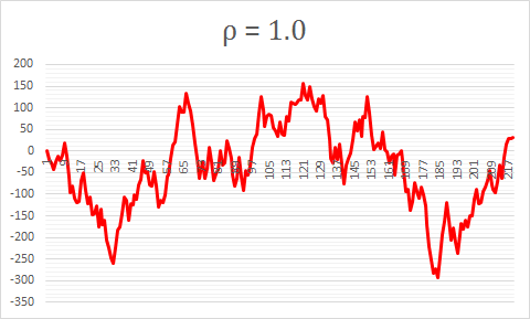
It is important to be aware that occasionally a purely random walk will, for periods of time ‘look like’ and exhibit the characteristics of a stationary process. Take a look at the following for ρ=1. This does not look dissimilar to the series for ρ=0.9 above. The series ‘appears’ to be somewhat mean reverting in nature. However, this is purely an illusion based on a specific set of random values. To infer that this stationary / mean reverting would not be true even though it might look like it is for the given time period. Take note: to avoid spurious regressions it is important that you only choose pairs that have been shown to exhibit stationarity repeatedly for periods in the past (as opposed to only for a recent observation).
Summary
Hopefully, you now have a good understanding of what stationarity is. This is good, since it is a key factor in being able to understand and determine if a pair of instruments is cointegrated.
In a future article, we may cover a test to formally and quantifiably identify stationarity using a technique called the Dickey-Fuller Test for cointegration.
